Relationships

# Relationships

**Session 7**

]

---

# Plan for today

.box-5.medium.sp-after-half[The dangers of dual y-axes]

.box-1.medium.sp-after-half[Visualizing correlations]

.box-6.medium.sp-after-half[Visualizing regressions]

---

name: dual-y-axes
class: center middle section-title section-title-5 animated fadeIn

# The dangers of dual y-axes

---

---

# Stop eating margarine!

.center[
<figure>
 <img src="img/07/chart.png" alt="Spurious correlation between divorce rate and margarine consumption" title="Spurious correlation between divorce rate and margarine consumption" width="100%">
 <figcaption>Source: <a href="https://www.tylervigen.com/spurious-correlations" target="_blank">Tyler Vigen's spurious correlations</a></figcaption>
</figure>
]

---

# Why not use double y-axes?

.box-inv-5.medium[You have to choose where the y-axes start and stop, which means…]

.box-inv-5.medium[…you can force the two trends to line up however you want!]

---

# It even happens in *The Economist!*

.center[
<figure>
 <img src="img/07/economist-dogs.png" alt="Dog neck size and weight in The Economist" title="Dog neck size and weight in The Economist" width="85%">
</figure>
]

???

<https://medium.economist.com/mistakes-weve-drawn-a-few-8cdd8a42d368>

---

# The rare triple y-axis!

.center[
<figure>
 <img src="img/07/triple-y-axis.png" alt="Acemoglu and Restrepo triple y-axis" title="Acemoglu and Restrepo triple y-axis" width="60%">
 <figcaption>Source: Daron Acemoglu and Pascual Restrepo, "The Race Between Man and Machine: Implications of Technology for Growth, Factor Shares and Employment"</figcaption>
</figure>
]

???

Daron Acemoglu and Pascual Restrepo, ["The Race Between Man and Machine: Implications of Technology for Growth, Factor Shares and Employment"](https://economics.mit.edu/files/10866)

---

# When is it legal?

.box-inv-5.medium[When the two axes measure the same thing]

.center[
<figure>
 <img src="img/07/3-operations.png" alt="Lollipop chart with dual y-axes from my dissertation" title="Lollipop chart with dual y-axes from my dissertation" width="85%">
</figure>
]

---

# When is it legal?

---

# Adding a second scale in R

```r
# From the uncertainty example
weather_atl <- 
 read_csv("data/atl-weather-2019.csv")

ggplot(weather_atl, 
       aes(x = time, y = temperatureHigh)) +
  geom_line() +
  geom_smooth() +
  scale_y_continuous(
    sec.axis = 
      sec_axis(trans = ~ (32 - .) * -5/9,
               name = "Celsius")
  ) +
  labs(x = NULL, y = "Fahrenheit")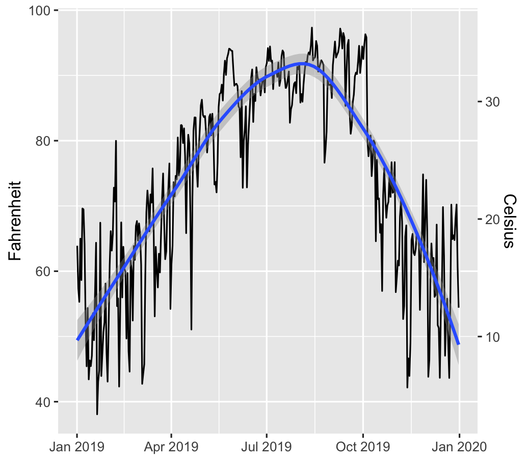
```
]

---

# Adding a second scale in R

```r
car_counts <- mpg %>% 
 group_by(drv) %>% 
 summarize(total = n())

total_cars <- sum(car_counts$total)

ggplot(car_counts,
       aes(x = drv, y = total, 
           fill = drv)) +
  geom_col() +
  scale_y_continuous(
    sec.axis = sec_axis(
      trans = ~ . / total_cars,
      labels = scales::percent)
  ) +
  guides(fill = "none")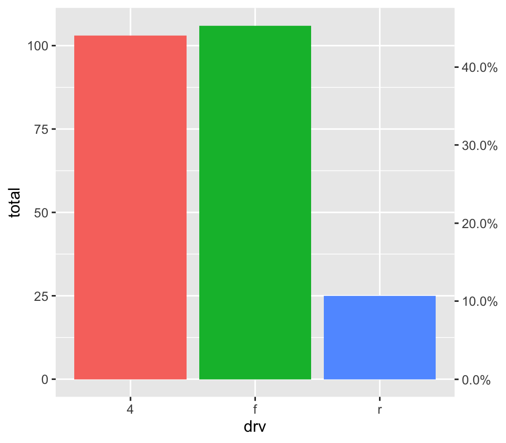
```
]

---

# Alternative 1: Use another aesthetic

.center[
<figure>
 <img src="img/03/gapminder-screenshot.png" alt="Animated gapminder data" title="Animated gapminder data" width="70%">
</figure>
]

---

# Alternative 2: Use multiple plots

.center[
<figure>
 <img src="img/07/timeline_HND.png" alt="Honduras anti-trafficking timeline" title="Honduras anti-trafficking timeline" width="65%">
 <figcaption>Anti-trafficking policy timeline in Honduras</figcaption>
</figure>
]

---

# Alternative 2: Use multiple plots

```r
library(patchwork)

temp_plot <- ggplot(weather_atl, 
 aes(x = time, 
 y = temperatureHigh)) +
 geom_line() + geom_smooth() +
 labs(x = NULL, y = "Fahrenheit")

humid_plot <- ggplot(weather_atl, 
 aes(x = time, 
 y = humidity)) +
 geom_line() + geom_smooth() +
 labs(x = NULL, y = "Humidity")

temp_plot + humid_plot +
  plot_layout(ncol = 1, 
              heights = c(0.7, 0.3))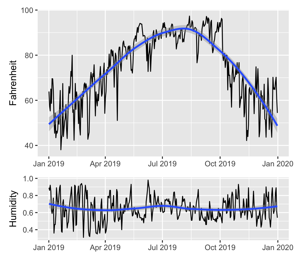
```
]

---

layout: false
name: correlation
class: center middle section-title section-title-1 animated fadeIn

# Visualizing correlations

---

---

# What is correlation?

.pull-right-wide[
.box-inv-1.medium[As the value of X goes up, Y tends to go up (or down) a lot/a little/not at all]

---

# Correlation values

<table>
 <tr>
 <th class="cell-left">r</th>
 <th class="cell-left">Rough meaning</th>
 </tr>
 <tr>
 <td class="cell-left">±0.1–0.3&emsp;</td>
 <td class="cell-left">Modest</td>
 </tr>
 <tr>
 <td class="cell-left">±0.3–0.5</td>
 <td class="cell-left">Moderate</td>
 </tr>
 <tr>
 <td class="cell-left">±0.5–0.8</td>
 <td class="cell-left">Strong</td>
 </tr>
 <tr>
 <td class="cell-left">±0.8–0.9</td>
 <td class="cell-left">Very strong</td>
 </tr>
</table>
]

]

---

# Scatterplot matrices

```r
library(GGally)

cars_smaller <- mtcars %>% 
 select(mpg, cyl, gear, hp, qsec)

ggpairs(cars_smaller)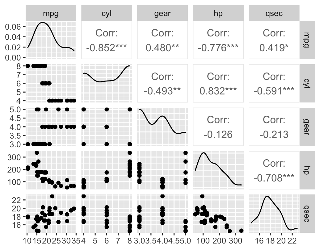
```
]

---

# Correlograms: Heatmaps

---

# Correlograms: Points

---

layout: false
name: regression
class: center middle section-title section-title-6 animated fadeIn

# Visualizing regressions

---

---

# Drawing lines

]

]

---

# Drawing lines with math

$$
y = mx + b
$$

<table>
 <tr>
 <td class="cell-center">$y$</td>
 <td class="cell-left">&ensp;A number</td>
 </tr>
 <tr>
 <td class="cell-center">$x$</td>
 <td class="cell-left">&ensp;A number</td>
 </tr>
 <tr>
 <td class="cell-center">$m$</td>
 <td class="cell-left">&ensp;Slope ($\frac{\text{rise}}{\text{run}}$)</td>
 </tr>
 <tr>
 <td class="cell-center">$b$</td>
 <td class="cell-left">&ensp;y-intercept</td>
 </tr>
</table>

---

# Slopes and intercepts

$$
y = 2x - 1
$$

]

$$
y = -0.5x + 6
$$

]

---

# Drawing lines with stats

$$
\hat{y} = \beta_0 + \beta_1 x_1 + \varepsilon
$$

<table>
 <tr>
 <td class="cell-center">$y$</td>
 <td class="cell-center">$\hat{y}$</td>
 <td class="cell-left">&ensp;Outcome variable (DV)</td>
 </tr>
 <tr>
 <td class="cell-center">$x$</td>
 <td class="cell-center">$x_1$</td>
 <td class="cell-left">&ensp;Explanatory variable (IV)</td>
 </tr>
 <tr>
 <td class="cell-center">$m$</td>
 <td class="cell-center">$\beta_1$</td>
 <td class="cell-left">&ensp;Slope</td>
 </tr>
 <tr>
 <td class="cell-center">$b$</td>
 <td class="cell-center">$\beta_0$</td>
 <td class="cell-left">&ensp;y-intercept</td>
 </tr>
 <tr>
 <td class="cell-center">&emsp;&emsp;</td>
 <td class="cell-center">&emsp;$\varepsilon$&emsp;</td>
 <td class="cell-left">&ensp;Error (residuals)</td>
 </tr>
</table>

---

# Building models in R

```r
name_of_model <- lm(<Y> ~ <X>, data = <DATA>)

summary(name_of_model)  # See model details
```

```r
library(broom)

# Convert model results to a data frame for plotting
tidy(name_of_model)

# Convert model diagnostics to a data frame
glance(name_of_model)
```

---

# Modeling displacement and MPG

```r
car_model <- lm(hwy ~ displ,
 data = mpg)
```

]

]

---

# Modeling displacement and MPG

```r
tidy(car_model, conf.int = TRUE)
```

```
## # A tibble: 2 x 7
## term estimate std.error statistic p.value conf.low conf.high
## <chr> <dbl> <dbl> <dbl> <dbl> <dbl> <dbl>
## 1 (Intercept) 35.7 0.720 49.6 2.12e-125 34.3 37.1 
## 2 displ -3.53 0.195 -18.2 2.04e- 46 -3.91 -3.15
```
]

```r
glance(car_model)
```

```
## # A tibble: 1 x 12
## r.squared adj.r.squared sigma statistic p.value df logLik AIC BIC
## <dbl> <dbl> <dbl> <dbl> <dbl> <dbl> <dbl> <dbl> <dbl>
## 1 0.587 0.585 3.84 329. 2.04e-46 1 -646. 1297. 1308.
## # … with 3 more variables: deviance <dbl>, df.residual <int>, nobs <int>
```
]

---

# Translating results to math

```
## # A tibble: 2 x 2
## term estimate
## <chr> <dbl>
## 1 (Intercept) 35.7 
## 2 displ -3.53
```
]

]

---

# Template for single variables

.box-inv-6.medium[A one unit increase in X is *associated* with a β1 increase (or decrease) in Y, on average]

$$
\hat{\text{hwy}} = \beta_0 + \beta_1 \text{displ} + \varepsilon
$$

$$
\hat{\text{hwy}} = 35.7 + (-3.53) \times \text{displ} + \varepsilon
$$

---

# Multiple regression

$$
\hat{y} = \beta_0 + \beta_1 x_1 + \beta_2 x_2 + \cdots + \beta_n x_n + \varepsilon
$$

&nbsp;

```r
car_model_big <- lm(hwy ~ displ + cyl + drv,
 data = mpg)
```

$$
\hat{\text{hwy}} = \beta_0 + \beta_1 \text{displ} + \beta_2 \text{cyl} + \beta_3 \text{drv:f} + \beta_4 \text{drv:r} + \varepsilon
$$

---

# Modeling lots of things and MPG

```r
tidy(car_model_big, conf.int = TRUE)
```

```
## # A tibble: 5 x 7
## term estimate std.error statistic p.value conf.low conf.high
## <chr> <dbl> <dbl> <dbl> <dbl> <dbl> <dbl>
## 1 (Intercept) 33.1 1.03 32.1 9.49e-87 31.1 35.1 
## 2 displ -1.12 0.461 -2.44 1.56e- 2 -2.03 -0.215
## 3 cyl -1.45 0.333 -4.36 1.99e- 5 -2.11 -0.796
## 4 drvf 5.04 0.513 9.83 3.07e-19 4.03 6.06 
## 5 drvr 4.89 0.712 6.86 6.20e-11 3.48 6.29
```
]

$$
`\begin{aligned}
\hat{\text{hwy}} =&\ 33.1 + (-1.12) \times \text{displ} + (-1.45) \times \text{cyl} \ + \\
&(5.04) \times \text{drv:f} + (4.89) \times \text{drv:r} + \varepsilon
\end{aligned}`
$$

---

# Sliders and switches

.center[
<figure>
 <img src="img/07/slider-switch-plain-80.jpg" alt="Switch and slider" title="Switch and slider" width="100%">
</figure>
]

---

# Sliders and switches

.center[
<figure>
 <img src="img/07/slider-switch-annotated-80.jpg" alt="Switch and slider" title="Switch and slider" width="100%">
</figure>
]

---

# Template for continuous variables

.box-inv-6[*Holding everything else constant*, a one unit increase in X is *associated* with a βn increase (or decrease) in Y, on average]

$$
`\begin{aligned}
\hat{\text{hwy}} =&\ 33.1 + (-1.12) \times \text{displ} + (-1.45) \times \text{cyl} \ + \\
&(5.04) \times \text{drv:f} + (4.89) \times \text{drv:r} + \varepsilon
\end{aligned}`
$$

.box-6.small[On average, a one unit increase in cylinders is associated with 1.45 lower highway MPG, holding everything else constant]

---

# Template for categorical variables

.box-inv-6[*Holding everything else constant*, Y is βn units larger (or smaller) in Xn, compared to Xomitted, on average]

$$
`\begin{aligned}
\hat{\text{hwy}} =&\ 33.1 + (-1.12) \times \text{displ} + (-1.45) \times \text{cyl} \ + \\
&(5.04) \times \text{drv:f} + (4.89) \times \text{drv:r} + \varepsilon
\end{aligned}`
$$

.box-6[On average, front-wheel drive cars have 5.04 higher highway MPG than 4-wheel-drive cars, holding everything else constant]

---

# Good luck visualizng all this!

&nbsp;

.box-inv-6.medium[You can't just draw a line! There are too many moving parts!]

---

# Main problems

.box-6.sp-after[Solution: Plot the coefficients and their errors with a *coefficient plot*]

---

# Coefficient plots

```r
car_model_big <- lm(hwy ~ displ + cyl + drv, data = mpg)

car_coefs <- tidy(car_model_big, conf.int = TRUE) %>% 
 filter(term != "(Intercept)") # We can typically skip plotting the intercept, so remove it
car_coefs
```

```
## # A tibble: 4 x 7
## term estimate std.error statistic p.value conf.low conf.high
## <chr> <dbl> <dbl> <dbl> <dbl> <dbl> <dbl>
## 1 displ -1.12 0.461 -2.44 1.56e- 2 -2.03 -0.215
## 2 cyl -1.45 0.333 -4.36 1.99e- 5 -2.11 -0.796
## 3 drvf 5.04 0.513 9.83 3.07e-19 4.03 6.06 
## 4 drvr 4.89 0.712 6.86 6.20e-11 3.48 6.29
```
]

---

# Coefficient plots

```r
ggplot(car_coefs,
       aes(x = estimate, 
           y = fct_rev(term))) +
  geom_pointrange(aes(xmin = conf.low, 
                      xmax = conf.high)) +
  geom_vline(xintercept = 0, color = "red")
```
]

---

# Marginal effects plots

.box-6.small.sp-after[We move one slider while leaving all the other sliders and switches alone]

.box-6.small[Plug a bunch of values into the model and find the predicted outcome]

.box-6.small[Plot the values and predicted outcome]

---

# Marginal effects plots

.box-inv-6[Create a data frame of values you want to manipulate and values you want to hold constant]

---

# Marginal effects plots

```r
cars_new_data <- tibble(displ = seq(2, 7, by = 0.1),
 cyl = mean(mpg$cyl),
 drv = "f")

head(cars_new_data)
```

```
## # A tibble: 6 x 3
## displ cyl drv 
## <dbl> <dbl> <chr>
## 1 2 5.89 f 
## 2 2.1 5.89 f 
## 3 2.2 5.89 f 
## 4 2.3 5.89 f 
## 5 2.4 5.89 f 
## 6 2.5 5.89 f
```
]

---

# Marginal effects plots

```r
predicted_mpg <- augment(car_model_big, newdata = cars_new_data,
 se_fit = TRUE)

head(predicted_mpg)
```

```
## # A tibble: 6 x 5
## displ cyl drv .fitted .se.fit
## <dbl> <dbl> <chr> <dbl> <dbl>
## 1 2 5.89 f 27.3 0.644
## 2 2.1 5.89 f 27.2 0.604
## 3 2.2 5.89 f 27.1 0.566
## 4 2.3 5.89 f 27.0 0.529
## 5 2.4 5.89 f 26.9 0.494
## 6 2.5 5.89 f 26.8 0.460
```
]

---

# Marginal effects plots

.box-6.small[Cylinders held at their mean; assumes front-wheel drive]

```r
ggplot(predicted_mpg,
       aes(x = displ, y = .fitted)) +
  geom_ribbon(aes(ymin = .fitted + 
                    (-1.96 * .se.fit),
                  ymax = .fitted + 
                    (1.96 * .se.fit)),
              fill = "#5601A4", 
              alpha = 0.5) +
  geom_line(size = 1, color = "#5601A4")
```
]

---

# Multiple effects at once

.box-6[What's the marginal effect of increasing displacement across the front-, rear-, and four-wheel drive cars?]

---

# Multiple effects at once

.box-inv-6[Create a new dataset with varying displacement *and* varying drive, holding cylinders at its mean]

---

# Multiple effects at once

```r
cars_new_data_fancy <- expand_grid(displ = seq(2, 7, by = 0.1),
 cyl = mean(mpg$cyl),
 drv = c("f", "r", "4"))

head(cars_new_data_fancy)
```

```
## # A tibble: 6 x 3
## displ cyl drv 
## <dbl> <dbl> <chr>
## 1 2 5.89 f 
## 2 2 5.89 r 
## 3 2 5.89 4 
## 4 2.1 5.89 f 
## 5 2.1 5.89 r 
## 6 2.1 5.89 4
```
]

---

# Multiple effects at once

```r
predicted_mpg_fancy <- augment(car_model_big, newdata = cars_new_data_fancy,
 se_fit = TRUE)

head(predicted_mpg_fancy)
```

```
## # A tibble: 6 x 5
## displ cyl drv .fitted .se.fit
## <dbl> <dbl> <chr> <dbl> <dbl>
## 1 2 5.89 f 27.3 0.644
## 2 2 5.89 r 27.2 1.14 
## 3 2 5.89 4 22.3 0.805
## 4 2.1 5.89 f 27.2 0.604
## 5 2.1 5.89 r 27.1 1.10 
## 6 2.1 5.89 4 22.2 0.763
```
]

---

# Multiple effects at once

.box-6.small[Cylinders held at their mean; colored/filled by drive]

```r
ggplot(predicted_mpg_fancy,
       aes(x = displ, y = .fitted)) +
  geom_ribbon(aes(ymin = .fitted + 
                    (-1.96 * .se.fit),
                  ymax = .fitted + 
                    (1.96 * .se.fit),
                  fill = drv),
              alpha = 0.5) +
  geom_line(aes(color = drv), size = 1)
```
]

---

# Multiple effects at once

.box-6.small[Cylinders held at their mean; colored/filled/facetted by drive]

---

# Not just OLS!

---

# Any type of statistical model

.box-6.small[Logistic, probit, and multinomial regression (ordered and unordered)]

.box-6.small[Multilevel (i.e. mixed and random effects) regression]

.box-6.small[Bayesian models (These are extra pretty with the [**tidybayes** package](https://github.com/mjskay/tidybayes))]

.box-6.small.sp-after[Machine learning models]

.box-inv-6[If it has coefficients and/or if it makes predictions, you can (and should) visualize it!]